
The Raiser's Edge Data Cleanup Series: Almighty Vlookup
Published
Hello Ladies and Gentlemen, and welcome back to our series on cleaning up data inside The Raiser's Edge. Only... sometimes this doesn't happen inside The Raiser's Edge.
Having used The Raiser's Edge for a great deal of time, I've handled a number of pretty massive data cleanup tasks. But I have a confession: no matter how much I love the features inside The Raiser's Edge (and anyone who has taken a class with me has heard me rattle off a top-10 list), nothing will ever steal my heart like a simple Excel function called vlookup.
As I usually do, we begin with a story: Once upon a time there was a gangly box office manager in charge of two databases: one was for his theatre's ticketing and subscriptions (The Patron Edge - PE) and the other for development and marketing data (The Raiser's Edge - RE). While the same constituents existed in each database, sometimes he would need reports or mailings using a little bit from PE and a little bit from RE.
Now, there were 2 ways to approach this problem: He could manually copy and paste all of this data together, to have everything in a single Excel document. Or, instead of wasting hours with copy and paste (for there were 112,000 records, so that would take forever), he could use the Almighty Vlookup.
(The box office manager was me. Twist.)
Here's the general overview of how this works. As an example, you have a list of volunteer event assignments you want to link to the constituent's contact info. You want to combine the information into a single table. This won't be a problem at all, as long as one thing is true: you will need to have something in common between the two. Observe:
Table 1:
Table 2:
What do these two tables have in common? It is their unique ID number on the left hand column. By having something in common (the fancy Computer Science term is a Key), you can stitch these two lists together by using the vlookup.
Now, hopefully you're already familiar with Excel functions. As for vlookup, I learned it through many, many, many fits and starts and failures and, eventually, successes. And I can say that no single tool saved me as much time over the years as did vlookup, which I regularly used hundreds of times a day. Let's take a look at how vlookup is structured:
VLOOKUP(lookup_value,table_array,col_index_num,range_lookup)
Ok, don't freak out, I'm gonna walk you through this. In fact, I'm going to start by translating it into normal English, or at least as normal as I know:
VLOOKUP(unique value, Table 2, Which column?, FALSE)
...That may not have helped. Let's dive in:
Lookup Value / Unique Value: First, you tell the system what these two tables have in common. In our case, it will be the unique ID Number (typically, Constituent ID).
Table_Array: This basically asks, of your two tables, where is the second table located? I have a neat timesaver to help with this step.
Col_index_number: Vlookup is amazing, but you already know that. It is amazing because when we stitch those two tables together, we decide which column from Table 2 we want to merge into Table 1. This is just a number indicating which column you want to merge. 1 would get you the first column, 2 would get you the second column, 3... you can probably deduce from there.
Range_lookup: Vlookup ends with an easy one: this is FALSE. Always just type FALSE. This will always be FALSE, just as I've been writing it here.
Now, I mentioned a nice time-saving tool above, and here it is: to simplify your life tremendously, we are going to select all of the data in Table 2 (not the header row in row 1!), right-click, and select "Name a Range".
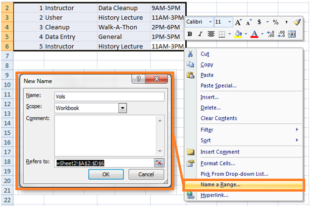
This is going to convert what Excel sees (=Sheet2!$A$2:$D$6) to something much easier to use ("Vols", or whatever you want to call it). Trust me when I say this is going to really make your life easier.
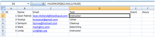
Now that our table 2 is renamed to Vols, we can get to work. I will go back to Table 1, and select cell D2, which is the same row as our data, but in the first blank column. Then I typed in our formula:
=VLOOKUP($A2,Vols,2,FALSE)
$A2: Remember we start by looking up the unique value, which for this user is in cell A2. Now, I'm going to strongly suggest that you put a $ before the cell... as this will make your life easier in a moment when we copy and paste.
Vols: Table 2, that we renamed above.
2: In this column, I want to return the "Task" column from Table 2, which is in column, you guessed it, number 2.
FALSE: It's always False.
Then, once I have this formula in D2, I copy and paste it to the remainder of the D column. Then, I figure it must be easy to copy and paste that formula into columns E and F as well, and I get:
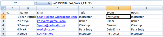
Hmm, that's not what I was looking for. Let's see why this could be. I have column E2 selected, and you can see the formula above. But notice which column we're returning? #2. Only, now we're looking for Event information which was in column.... 3. And Hours will be under column 4. So I need to change 2 to 3 and 4 (respectively).
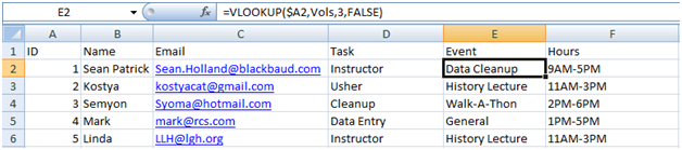
Now with those changes made, I copy and pasted over the remaining entries, and we are done.
Here's what my final data and formulas look like.
One final task: if you want just this data with the raw text (in other words, with the formulas stripped), copy all of your data, right-click where you want it to go, and click "Paste Special". Then select "values". This will ensure only your data survives, without the formulas.
I love vlookup, but as I alluded to above, it took me a long while to figure out exactly what was going on and how it could best be utilized. Basically, my best suggestion is: try it. You can copy Table 1 and Table 2 above and give it a whirl.
Some Best Practices:
One way or another, I found myself using vlookup to solve countless problems in my database. When I wanted to link our constituents to non-RE data, when I was hunting for duplicate records, when I was amassing large amounts of historical data, or when I was cleaning up my data. Remember, everything we learn in the system goes into our little metaphorical toolbox, and this is one of the best tools you can use.
There is most information on VLOOKUP and many other great Excel tips in the in-person class Preparing Data for Import with Microsoft Excel, which is then followed up with Advanced Importing Techniques in The Raiser's Edge. For more information on importing for online classes, check out Fundamentals of Importing in The Raiser's Edge.
As always, if you have any suggestions for future posts, hit me in the comments! I wish you all luck, and I hope you will love vlookup as much as I do.
Having used The Raiser's Edge for a great deal of time, I've handled a number of pretty massive data cleanup tasks. But I have a confession: no matter how much I love the features inside The Raiser's Edge (and anyone who has taken a class with me has heard me rattle off a top-10 list), nothing will ever steal my heart like a simple Excel function called vlookup.
As I usually do, we begin with a story: Once upon a time there was a gangly box office manager in charge of two databases: one was for his theatre's ticketing and subscriptions (The Patron Edge - PE) and the other for development and marketing data (The Raiser's Edge - RE). While the same constituents existed in each database, sometimes he would need reports or mailings using a little bit from PE and a little bit from RE.
Now, there were 2 ways to approach this problem: He could manually copy and paste all of this data together, to have everything in a single Excel document. Or, instead of wasting hours with copy and paste (for there were 112,000 records, so that would take forever), he could use the Almighty Vlookup.
(The box office manager was me. Twist.)
Here's the general overview of how this works. As an example, you have a list of volunteer event assignments you want to link to the constituent's contact info. You want to combine the information into a single table. This won't be a problem at all, as long as one thing is true: you will need to have something in common between the two. Observe:
Table 1:
| ID | Name | |
| 1 | Sean Patrick | Sean.Holland@blackbaud.com |
| 2 | Kostya | kostyacat@gmail.com |
| 3 | Semyon | Syoma@hotmail.com |
| 4 | Mark | mark@rcs.com |
| 5 | Linda | LLH@lgh.org |
Table 2:
| ID | Task | Event | Hours |
| 1 | Instructor | Data Cleanup | 9AM-5PM |
| 2 | Usher | History Lecture | 11AM-3PM |
| 3 | Cleanup | Walk-A-Thon | 2PM-6PM |
| 4 | Data Entry | General | 1PM-5PM |
| 5 | Instructor | History Lecture | 11AM-3PM |
What do these two tables have in common? It is their unique ID number on the left hand column. By having something in common (the fancy Computer Science term is a Key), you can stitch these two lists together by using the vlookup.
Now, hopefully you're already familiar with Excel functions. As for vlookup, I learned it through many, many, many fits and starts and failures and, eventually, successes. And I can say that no single tool saved me as much time over the years as did vlookup, which I regularly used hundreds of times a day. Let's take a look at how vlookup is structured:
VLOOKUP(lookup_value,table_array,col_index_num,range_lookup)
Ok, don't freak out, I'm gonna walk you through this. In fact, I'm going to start by translating it into normal English, or at least as normal as I know:
VLOOKUP(unique value, Table 2, Which column?, FALSE)
...That may not have helped. Let's dive in:
Lookup Value / Unique Value: First, you tell the system what these two tables have in common. In our case, it will be the unique ID Number (typically, Constituent ID).
Table_Array: This basically asks, of your two tables, where is the second table located? I have a neat timesaver to help with this step.
Col_index_number: Vlookup is amazing, but you already know that. It is amazing because when we stitch those two tables together, we decide which column from Table 2 we want to merge into Table 1. This is just a number indicating which column you want to merge. 1 would get you the first column, 2 would get you the second column, 3... you can probably deduce from there.
Range_lookup: Vlookup ends with an easy one: this is FALSE. Always just type FALSE. This will always be FALSE, just as I've been writing it here.
Now, I mentioned a nice time-saving tool above, and here it is: to simplify your life tremendously, we are going to select all of the data in Table 2 (not the header row in row 1!), right-click, and select "Name a Range".
This is going to convert what Excel sees (=Sheet2!$A$2:$D$6) to something much easier to use ("Vols", or whatever you want to call it). Trust me when I say this is going to really make your life easier.
Now that our table 2 is renamed to Vols, we can get to work. I will go back to Table 1, and select cell D2, which is the same row as our data, but in the first blank column. Then I typed in our formula:
=VLOOKUP($A2,Vols,2,FALSE)
$A2: Remember we start by looking up the unique value, which for this user is in cell A2. Now, I'm going to strongly suggest that you put a $ before the cell... as this will make your life easier in a moment when we copy and paste.
Vols: Table 2, that we renamed above.
2: In this column, I want to return the "Task" column from Table 2, which is in column, you guessed it, number 2.
FALSE: It's always False.
Then, once I have this formula in D2, I copy and paste it to the remainder of the D column. Then, I figure it must be easy to copy and paste that formula into columns E and F as well, and I get:
Hmm, that's not what I was looking for. Let's see why this could be. I have column E2 selected, and you can see the formula above. But notice which column we're returning? #2. Only, now we're looking for Event information which was in column.... 3. And Hours will be under column 4. So I need to change 2 to 3 and 4 (respectively).
Now with those changes made, I copy and pasted over the remaining entries, and we are done.
Here's what my final data and formulas look like.
| ID | Name | Task | Event | Hours |
| 1 | Sean Patrick | =VLOOKUP($A2,Vols,2,FALSE) | =VLOOKUP($A2,Vols,3,FALSE) | =VLOOKUP($A2,Vols,4,FALSE) |
| 2 | Kostya | =VLOOKUP($A3,Vols,2,FALSE) | =VLOOKUP($A3,Vols,3,FALSE) | =VLOOKUP($A3,Vols,4,FALSE) |
| 3 | Semyon | =VLOOKUP($A4,Vols,2,FALSE) | =VLOOKUP($A4,Vols,3,FALSE) | =VLOOKUP($A4,Vols,4,FALSE) |
| 4 | Mark | =VLOOKUP($A5,Vols,2,FALSE) | =VLOOKUP($A5,Vols,3,FALSE) | =VLOOKUP($A5,Vols,4,FALSE) |
| 5 | Linda | =VLOOKUP($A6,Vols,2,FALSE) | =VLOOKUP($A6,Vols,3,FALSE) | =VLOOKUP($A6,Vols,4,FALSE) |
One final task: if you want just this data with the raw text (in other words, with the formulas stripped), copy all of your data, right-click where you want it to go, and click "Paste Special". Then select "values". This will ensure only your data survives, without the formulas.
I love vlookup, but as I alluded to above, it took me a long while to figure out exactly what was going on and how it could best be utilized. Basically, my best suggestion is: try it. You can copy Table 1 and Table 2 above and give it a whirl.
Some Best Practices:
- Ensure the unique values (keys) are in the left-most column
- Also ensure the keys are sorted in Ascending order
- Select your second table's data, then right-click and Name a Range to give it an easily-used title
- Add a $ before the unique value to make copy and pasting easier
- Once everything is done, Paste Special->Values to only get the data
One way or another, I found myself using vlookup to solve countless problems in my database. When I wanted to link our constituents to non-RE data, when I was hunting for duplicate records, when I was amassing large amounts of historical data, or when I was cleaning up my data. Remember, everything we learn in the system goes into our little metaphorical toolbox, and this is one of the best tools you can use.
There is most information on VLOOKUP and many other great Excel tips in the in-person class Preparing Data for Import with Microsoft Excel, which is then followed up with Advanced Importing Techniques in The Raiser's Edge. For more information on importing for online classes, check out Fundamentals of Importing in The Raiser's Edge.
As always, if you have any suggestions for future posts, hit me in the comments! I wish you all luck, and I hope you will love vlookup as much as I do.
News
Raiser's Edge® Blog
07/15/2013 8:49am EDT
Leave a Comment